Today we’ll look at how to efficiently render a large terrain in 3D. We’ll be using WebGL to do this, but the techniques can be applied pretty much anywhere.

We’ll concentrate on the vertex shader, that is, how best to use the position the vertices of our terrain mesh, so that it looks good up close as well as far away.

To see how this end result looks, check out the live demo. The demo was built using THREE.js, and the code is on github, if you’re interested in the details.

LOD - Level of detail

An important concept when rendering terrain is the “level of detail”. This describes how many vertices we are drawing in a particular region.

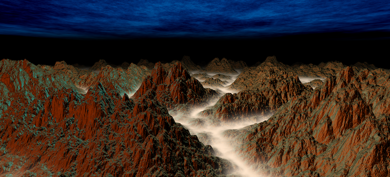
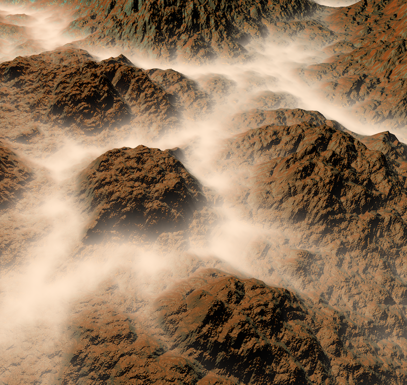
Take the terrain below, notice how the nearby mountain on the right fills a lot of the final image, while the mountains in the distance only take a small portion of the image.

It makes sense to render nearby objects with a greater LOD, while those in the distance with a lower LOD. This way we don’t waste processing power computing a thousand vertices that end up in the same pixel on screen.

Flat grid

An easy way to create a terrain mesh is to simply create a plane that covers our entire terrain, and sub-divide it into a uniform grid. This is pretty awful for the LOD, as distant features will have far too much detail, while those nearby not enough. As we add vertices to the uniform grid to improve the nearby features, we are wasting ever more on the distant features, while reducing the vertex count to bring down the vertices used to draw the distant features will impact the nearby features.

Recursive tiles

A simple way to do better is to split our plane into tiles of differing sizes, but of constant vertex count. So for example, each tile contains 64x64 vertices, but sometimes these vertices are stretched over an area corresponding to a large distant area, while for nearby areas, the tiles are smaller.

The question remains how to arrange these tiles. There are more sophisticated methods for doing this, but we’ll stick with something simpler. Specifically, we’ll start with the area nearest to the camera and fill it with tiles of the highest resolution, say 1x1. We’ll then surround this area with a “shell” of tiles of double the size, 2x2. We’ll then add a 4x4 tile “shell”, and so on, until we have covered our map. Here’s how this looks, with each layer color-coded:

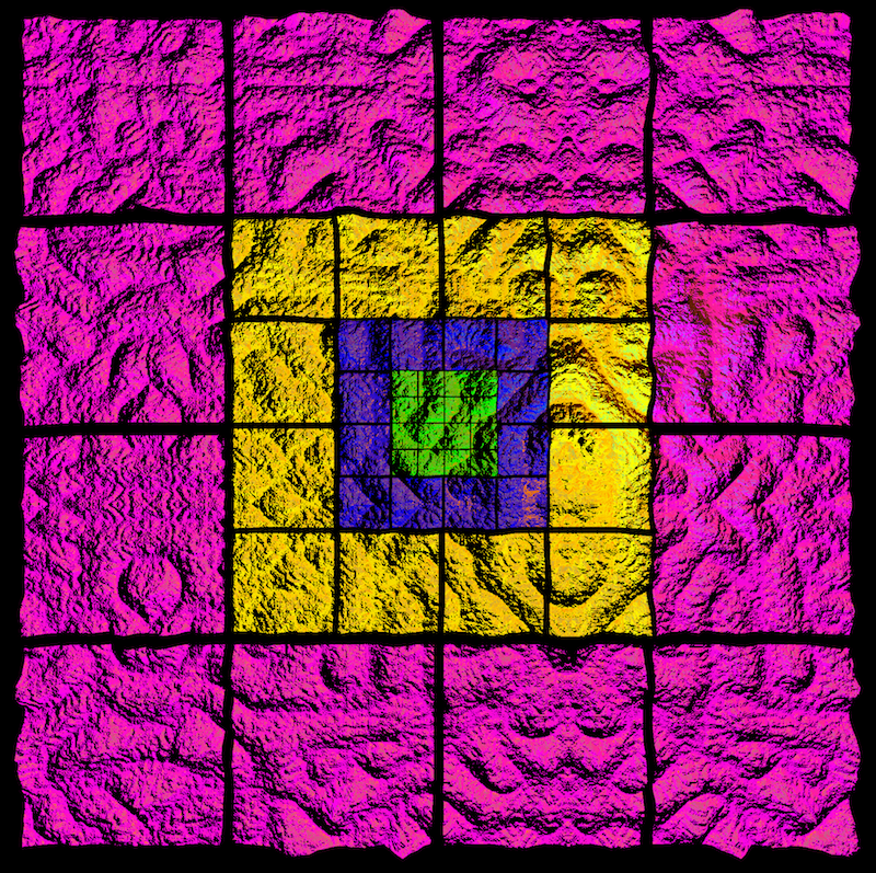
Notice how the central layer actually has 4 extra tiles than the others, this is necessary, otherwise we’d end up with a hole in the middle. This tile arrangement is actually very nice, as each additional “shell” doubles the width and height of the area covered, while only required a constant number of additional tiles.

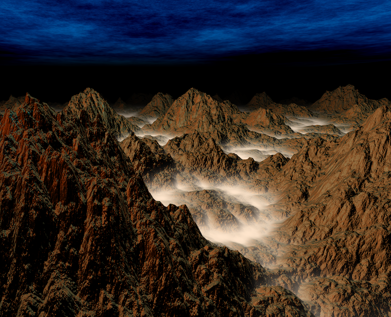
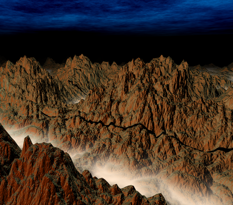
When viewed from above, this arrangement doesn’t seem particularly great, as all the tiles are more or less the same distance from the camera. However, a more usual view is one where the camera is pointed at the horizon and hence nearby tiles are filling more of the final view:

In this view it is clear that we’re already doing much better with our vertex distribution. Each “shell” is represented roughly equally in the final image, which means that our vertex density is roughly uniform across the image.

Moving around

Now that we have a suitable mesh, we need to address how what will happen as the camera moves around the terrain. One idea is to actually keep the mesh itself static, but let the terrain data “flow” through the mesh. Imagine that each vertex is part of a cloth that is being warped to the shape of the underlying terrain. As we move around the terrain, the cloth is dragged over it, being deformed into the correct shape below it.

The advantage of this approach is that we always have the correct LOD now matter where we move, as the terrain mesh is static relative to the camera.

The problem is that as the terrain “flows” through the mesh, if the vertices are not sufficiently close together, they will not do a good job of sampling the terrain, in particular they will wobble as the terrain flows through them.

To illustrate why this happens, consider a region of the terrain where the vertex spacing is large, e.g. 1km. Imagine that the terrain we are displaying has alternating valleys and hills at this point, spaced 1km apart. As the terrain “flows” thorough the mesh, then sometimes the vertices will all be on the hills and other times they will be in the valleys. Now as this is a region that is far from the camera, we don’t care so much that the hills and valleys aren’t shown correctly, as either alone would be fine. The real issue is that the oscillation between the two creates flickering, which is visually distracting.

Grid snapping

To solve this oscillation issue, we keep the same geometry as we had before, except that we make it so that when the terrain “flows” through the mesh, the vertices snap to a grid, with spacing equal to the vertex spacing for that tile. So in the hill/valley example from before, rather than having a vertex “flow” from the top of the hill to the bottom of the valley and then back up, it is instead snapped to the nearest hill-top. By making the snap grid be spaced at the same interval as the tiles vertex spacing, we will end up with a uniform grid again, except snapped to a fixed point on the terrain.

Morphing between regions

Ok, so we’ve solved one problem, but now we’re faced with another. As we’re snapping each tile according to it’s vertex spacing, where two tile layers meet we end up with seams, as shown below:

To fix this we want to gradually blend one layer into another, so that we end up with a continuous mesh. One way to do this is to compute what we’ll call a “morph factor”, which determines how close we are to the boundary between two different LOD layers. When we are near the boundary with a layer that has a greater vertex spacing than ours, the value of the morph factor approaches 1, while when we are far away, it is 0.

We can then use this value to blend smoothly between one layer and the other. The way we do this is calculate what the position of the vertex would be if it were snapped to both it’s own grid and that of the next layer and then linearly blend the two positions according to the morph factor. Here’s some GLSL code that does just that:

// Snap to grid
float grid = uScale / TILE_RESOLUTION;
vPosition = floor(vPosition / grid) * grid;

// Morph between zoom layers
if ( vMorphFactor > 0.0 ) {
  // Get position that we would have if we were on higher level grid
  grid = 2.0 * grid;
  vec3 position2 = floor(vPosition / grid) * grid;

  // Linearly interpolate the two, depending on morph factor
  vPosition = mix(vPosition, position2, vMorphFactor);
}

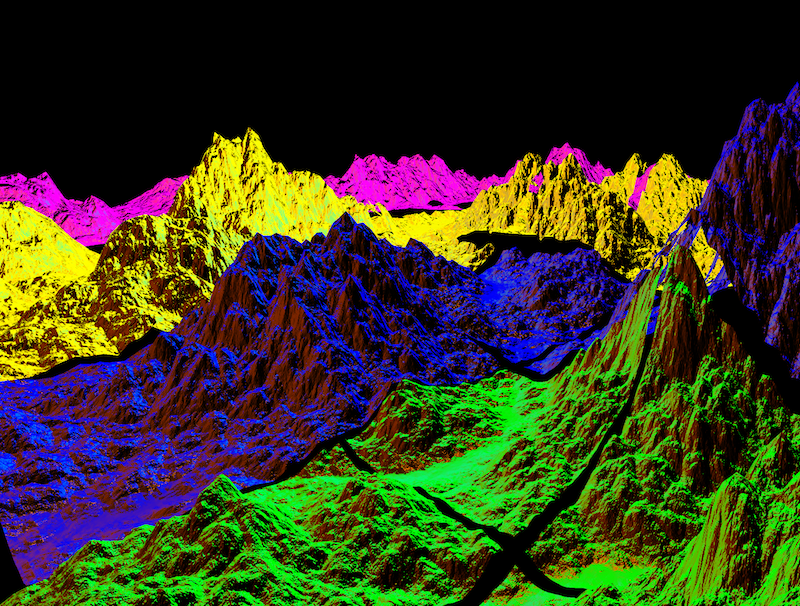
Here’s the terrain with the areas where the morph factor is non-zero highlighted in white.

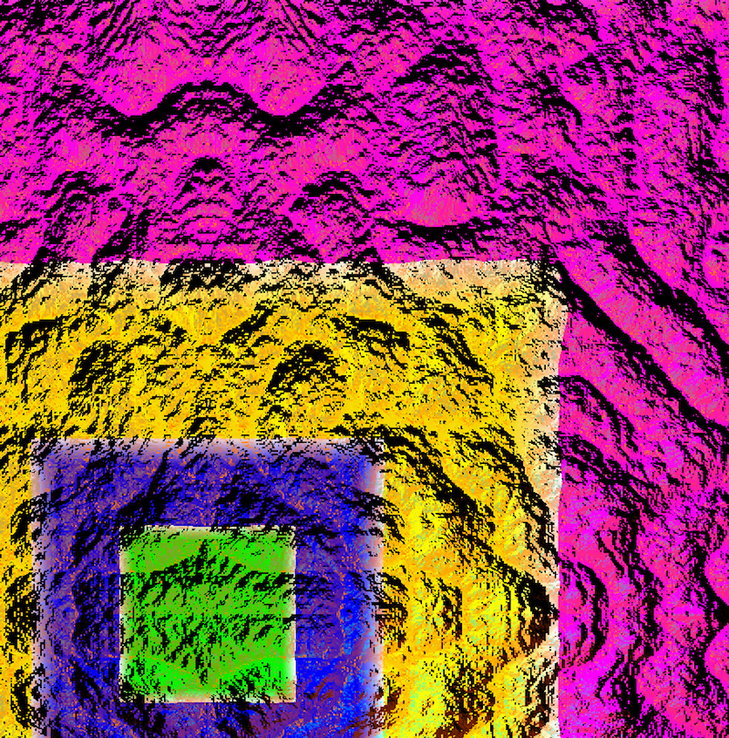
As before, each tile shell is color coded. Notice how each tile becomes completely white on the boundary with the next shell - as it morphs to have the same vertex spacing as the neighbouring tile.

Live demo

To see the terrain in action, check out the demo. The resolution of the tiles has been chosen such that it is hard to notice the transitions between different levels of detail. If you look closely though, at a distant mountain as it comes closer, you should be able to spot the terrain gradually blending into a higher-vertex representation. The source is on github if you want to play around with parameters to change the look or color of the terrain.

Finally, some of the ideas in this post were taken from the CDLOD paper, which is well worth a read.